Introduciton
In this post I show how to make a nice looking SEM diagram from a model object fitted with lavaan.
library(tidyverse)
library(lavaan)
library(ggnetwork)
Lavaan Model
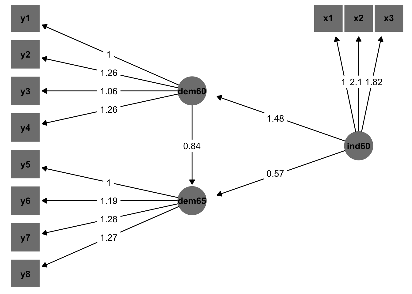
Below is the SEM model we are going to fit (from the lavaan website).
# Lavaan Model
model <- '
  # measurement model
    ind60 =~ x1 + x2 + x3
    dem60 =~ y1 + y2 + y3 + y4
    dem65 =~ y5 + y6 + y7 + y8
  # regressions
    dem60 ~ ind60
    dem65 ~ ind60 + dem60
  # residual correlations
    y1 ~~ y5
    y2 ~~ y4 + y6
    y3 ~~ y7
    y4 ~~ y8
    y6 ~~ y8
'
fit <- sem(model, data=PoliticalDemocracy)
Here is the output:
summary(fit, standardized=TRUE)## lavaan 0.6-9 ended normally after 68 iterations
##
## Estimator ML
## Optimization method NLMINB
## Number of model parameters 31
##
## Number of observations 75
##
## Model Test User Model:
##
## Test statistic 38.125
## Degrees of freedom 35
## P-value (Chi-square) 0.329
##
## Parameter Estimates:
##
## Standard errors Standard
## Information Expected
## Information saturated (h1) model Structured
##
## Latent Variables:
## Estimate Std.Err z-value P(>|z|) Std.lv Std.all
## ind60 =~
## x1 1.000 0.670 0.920
## x2 2.180 0.139 15.742 0.000 1.460 0.973
## x3 1.819 0.152 11.967 0.000 1.218 0.872
## dem60 =~
## y1 1.000 2.223 0.850
## y2 1.257 0.182 6.889 0.000 2.794 0.717
## y3 1.058 0.151 6.987 0.000 2.351 0.722
## y4 1.265 0.145 8.722 0.000 2.812 0.846
## dem65 =~
## y5 1.000 2.103 0.808
## y6 1.186 0.169 7.024 0.000 2.493 0.746
## y7 1.280 0.160 8.002 0.000 2.691 0.824
## y8 1.266 0.158 8.007 0.000 2.662 0.828
##
## Regressions:
## Estimate Std.Err z-value P(>|z|) Std.lv Std.all
## dem60 ~
## ind60 1.483 0.399 3.715 0.000 0.447 0.447
## dem65 ~
## ind60 0.572 0.221 2.586 0.010 0.182 0.182
## dem60 0.837 0.098 8.514 0.000 0.885 0.885
##
## Covariances:
## Estimate Std.Err z-value P(>|z|) Std.lv Std.all
## .y1 ~~
## .y5 0.624 0.358 1.741 0.082 0.624 0.296
## .y2 ~~
## .y4 1.313 0.702 1.871 0.061 1.313 0.273
## .y6 2.153 0.734 2.934 0.003 2.153 0.356
## .y3 ~~
## .y7 0.795 0.608 1.308 0.191 0.795 0.191
## .y4 ~~
## .y8 0.348 0.442 0.787 0.431 0.348 0.109
## .y6 ~~
## .y8 1.356 0.568 2.386 0.017 1.356 0.338
##
## Variances:
## Estimate Std.Err z-value P(>|z|) Std.lv Std.all
## .x1 0.082 0.019 4.184 0.000 0.082 0.154
## .x2 0.120 0.070 1.718 0.086 0.120 0.053
## .x3 0.467 0.090 5.177 0.000 0.467 0.239
## .y1 1.891 0.444 4.256 0.000 1.891 0.277
## .y2 7.373 1.374 5.366 0.000 7.373 0.486
## .y3 5.067 0.952 5.324 0.000 5.067 0.478
## .y4 3.148 0.739 4.261 0.000 3.148 0.285
## .y5 2.351 0.480 4.895 0.000 2.351 0.347
## .y6 4.954 0.914 5.419 0.000 4.954 0.443
## .y7 3.431 0.713 4.814 0.000 3.431 0.322
## .y8 3.254 0.695 4.685 0.000 3.254 0.315
## ind60 0.448 0.087 5.173 0.000 1.000 1.000
## .dem60 3.956 0.921 4.295 0.000 0.800 0.800
## .dem65 0.172 0.215 0.803 0.422 0.039 0.039Create Nodes
Now we are going to create a nice data.frame to specify the locations of nodes (variables in the SEM model) and edges (paths connecting nodes). First, define where the nodes should be positioned spatially and create a data.frame to hold these data:
lavaan_parameters <- parameterestimates(fit)

nodes <- lavaan_parameters %>%
  select(lhs) %>%
  rename(name = lhs) %>%
  distinct(name) %>%
  mutate(
    x = case_when(str_detect(name,("^y"))      ~ 0,
                  name %in% c("dem60","dem65") ~ .33,
                  name == "ind60"              ~ .66,
                  name == "x1"                 ~ .6,
                  name == "x2"                 ~ .66,
                  name == "x3"                 ~ .72),
    y = case_when(name %in% c("x1","x2","x3")       ~ 1.05,
                  name == "y1"                      ~ 1.05,
                  name == "y2"                      ~ .9,
                  name %in% c("y3","dem60")         ~ .75,
                  name == "ind60"                   ~ .525,
                  name == "y4"                      ~ .6,
                  name == "y5"                      ~ .45,
                  name %in% c("y6","dem65")         ~ .3,
                  name == "y7"                      ~ .15,
                  name == "y8"                      ~  0),
    xend = x,
    yend = y
  )
Create Edges
Now the same for edges:
edges <- lavaan_parameters %>%
  filter(op %in% c("~","=~"))
Next we need to combine our nodes and edges into a single table so we can plot it with ggplot2. To do this, we will merge the nodes and edges in a specific way to get all information represented in a single data.frame:
combined <- nodes %>%
  bind_rows(
    left_join(edges,nodes %>% select(name,x,y),by=c("lhs"="name")) %>%
      left_join(nodes %>% select(name,xend,yend),by = c("rhs"="name"))
  )

combined_edge_labels <- combined %>%
  mutate(
    est = round(est,2),
    p.code     = ifelse(pvalue<.05,"p < .05","p > .05"),
    shape      = ifelse(str_detect(name,"y\\d|x\\d"),"observed","latent"),
    midpoint.x = (x + xend)/2,
    midpoint.y = (y + yend)/2,
    x2    = ifelse(op=="~",xend,x),
    xend2 = ifelse(op=="~",x,xend),
    y2    = ifelse(op=="~",yend,y),
    yend2 = ifelse(op=="~",y,yend),
    rise = yend2-y2,
    run  = x2-xend2,
    dist = sqrt(run^2 + rise^2) %>% round(2),
    newx = case_when(str_detect(rhs,"y\\d") ~ (x2 + (xend2 - x2) * .90),
                     str_detect(rhs,"x\\d") ~ (x2 + (xend2 - x2) * .75),
                     lhs == "dem65" & rhs == "dem60" ~ (x2 + (xend2 - x2) * .7),
                     lhs == "dem65" & rhs == "ind60" ~ (x2 + (xend2 - x2) * .85),
                     lhs == "dem60" & rhs == "ind60" ~ (x2 + (xend2 - x2) * .85)),
    newy = case_when(str_detect(rhs,"y\\d") ~ (y2 + (yend2 - y2) * .90),
                     str_detect(rhs,"x\\d") ~ (y2 + (yend2 - y2) * .85),
                     lhs == "dem65" & rhs == "dem60" ~ (y2 + (yend2 - y2) * .85),
                     lhs == "dem65" & rhs == "ind60" ~ (y2 + (yend2 - y2) * .9),
                     lhs == "dem60" & rhs == "ind60" ~ (y2 + (yend2 - y2) * .9)),
  )
Make the Diagram
Now we plot:
combined_edge_labels %>%
  ggplot(aes(x = x, y = y, xend = xend, yend = yend)) +
  geom_edges(aes(x = x2, y = y2, xend = newx, yend = newy),
             arrow = arrow(length = unit(6, "pt"), type = "closed",ends = "last")) +
  geom_nodes(aes(shape = factor(shape,levels = c("observed","latent"))), color = "grey50",size = 16) +
  geom_nodetext(aes(label = name),fontface = "bold") +
  geom_label(aes(x = midpoint.x, y = midpoint.y, label = est), color = "black",label.size = NA,hjust = .5,vjust=.5) +
  scale_y_continuous(expand = c(.05,0)) +
  scale_shape_manual(values = c(15,19),guide=F) +
  theme_blank()