Introduction
In recent years, there is a growing interest in multiverse analysis, a technique for compiling all possible datasets that could result from different data processing decisions. Once compiled, researchers can run their analysis of interest across all datasets in the multiverse to see how sensitive their models are to the decisions that produced the underlying data. In this post, I attempt my own multiverse analysis using simulated data.
Note that there are already many good places to learn more about the multiverse analysis, including papers, blog posts, and code examples. My intention is to understand the mechanics of the technique without the aid of a pre-written package. My goal is to deepen my own understanding and to flesh out the different ways to use the technique and compile/visualize the results.
Arbitrary vs. Non-Arbitrary Decisions
Processing raw data involves many steps, such as cleaning, preparing, and creating analysis variables (among many others). Such decisions eventually produce an analysis-ready dataset, but making (even slightly) different decisions will produce a different dataset. And so emerges the multiverse: all possible datasets that could be generated from different data processing decisions (see also the garden of forking paths).
An important distinction in multiverse analysis is between arbitrary and non-arbitrary decisions. Arbitrary decisions are those that:
- are not expected to influence results (or their effect is unknown) and,
- equally defensible/have reasonable justifications
For example, whether to remove outliers at +/- 3 or 2.5 standard deviations could be arbitrary. Neither cutoff is theoretically informed and both are equally defensible.
In contrast, non-arbitrary choices are expected to affect results, either for theoretical or empirical reasons. For example, theory might suggest controlling for a confound is crucial for interpreting results. Empirically, controlling for a confound may aid interpretation because such a confound is known to correlate with the outcome of interest and should be accounted for in our analysis.
Multiverse analysis should be ran over all possible arbitrary decisions. This is important because the multiverse can quickly become unnecessarily large and difficult to interpret. Ideally, the multiverse will comprise all datasets that, by themselves, would make sense to analyze and interpret individually.
Setup
To conduct my multiverse analysis, I will be using a number of packages from the tidyverse. Below are the specific packages I used for my setup:
# Load relevant libraries
library(tidyverse)
library(lmerTest)
library(broom.mixed)
library(tidymodels)
library(ggeffects)
library(interactions)
library(effectsize)
library(showtext)
library(furrr)
# Custom font for ggplot
font_add_google("Lato")
showtext_auto()
# Set the ggplot2 theme
theme_set(
  theme_light() +
    theme(
      text = element_text(family="Lato"),
      panel.grid = element_blank()
    )
)
Simulated Data
The raw data are randomly generated below. I modeled the variables based on an actual project I am working on. The research question is whether or not early life unpredictability1 (iv_unp) is associated with performance on a cognitive test with two versions, a standard (dv_std) and ecologically relevant (dv_eco) version2. We hypothesize that unpredictability negatively impacts performance on the standard version but enhances performance on the ecological version. To that end, I’ve made performance depend on iv_unp with some error.
Exclusion variables are also included in the data.
ex_sample: The data (not these but those that I will be actually analyzing in a real dataset) come from two samples. The first sample is smaller and considerably more difficult to run our protocol. The second sample is larger and was much easier to control how the protocol was executed. Thus our results could be different depending on whether or not we include the smaller, noisier sample.ex_csd: socially desirable responding, which may have undue influence on our predictor. Children who experience adversity, and might want to hide it, may also score high on a measure of socially desirability.ex_sped: Some in our sample receive special education. It is possible that some students may have cognitive impairments and shouldn’t be analyzed with rest or the sample.ex_att: We included an a few trap questions in our assessment to detect individuals who may not be taking the study seriously.ex_imp: Our research assistants noted whether or not participants had trouble reading or seemed impaired somehow.
These variables will be used to construct a multiverse of datasets.
# Set the seed for reproducibility
set.seed(12345)
# detect cores for parrallel processing
cores <- parallel::detectCores()
# Create some data
sim_data <-
  tibble(
    id          = 1:500,
    intercept   = rnorm(500, mean = 0, sd = 3),
    iv_unp      = rnorm(500, mean = 0, sd = 1),
    ex_sample   = rbinom(500, size = 1, prob = .2),
    ex_csd      = rnorm(500, mean = 0, sd = 1) + iv_unp * (.15) + rnorm(500, mean = 0, 1),
    ex_sped     = rbinom(500, size = 1, prob = .1),
    ex_att      = rbinom(500, size = 1, prob = .1),
    ex_imp      = rbinom(500, size = 1, prob = .05)
  ) %>%
  mutate(
    intercept   = ifelse(ex_sped == 1, intercept - rnorm(1,.5,.25), intercept),
    intercept   = ifelse(ex_imp == 1, intercept - rnorm(1,.5,.25), intercept),
    intercept   = ifelse(ex_att == 1, intercept - rnorm(1,.25,.25), intercept),
    dv_std      = intercept + iv_unp * -(.2) + rnorm(500, mean = 0, 2),
    dv_eco      = intercept + iv_unp *  (.1) + rnorm(500, mean = 0, 2)
  )
And here are the first 10 rows of the simulated data:
| id | iv_unp | dv_std | dv_eco | ex_sample | ex_csd | ex_sped | ex_att | ex_imp |
|---|---|---|---|---|---|---|---|---|
| 1 | -1.42 | 2.02 | 5.05 | 1 | 2.07 | 0 | 0 | 0 |
| 2 | -2.47 | 4.82 | 4.53 | 0 | 1.65 | 0 | 0 | 0 |
| 3 | 0.48 | 1.49 | -0.08 | 0 | 1.19 | 0 | 0 | 0 |
| 4 | -0.94 | -2.27 | -5.54 | 1 | 0.43 | 0 | 0 | 0 |
| 5 | 3.33 | 0.23 | 2.36 | 0 | 0.71 | 0 | 0 | 0 |
| 6 | -0.16 | -4.52 | -4.39 | 1 | 1.44 | 0 | 0 | 0 |
The Arbitrary Data Decision Grid
The first step in conducting creating a multiverse is to construct a grid of data-filtering and/or processing decisions. The function expand_grid() creates all possible combinations of these decisions. My decisions are as follows:
- Include or exclude the smaller subsample
- Include or exclude people who failed attention checks
- Include or exclude participants with impairments
- Include or exclude special education status
- Include all scores, only scores > -3 SDs, or scores > -2.5 SDs
- Do nothing with social desirability, residualize
ex_csdfromiv_unp, or includeex_csdas a covariate
decision_grid <-
  expand_grid(
    ex_sample    = c("ex_sample %in% c(0,1)", "ex_sample == 0"),
    ex_att       = c("ex_att %in% c(0,1)",    "ex_att == 0"),
    ex_imp       = c("ex_imp %in% c(0,1)",    "ex_imp == 0"),
    ex_sped      = c("ex_sped %in% c(0,1)",   "ex_sped == 0"),
    dv_std       = c("scale(dv_std) > -10", "scale(dv_std) > -3", "scale(dv_std) > -2.5"),
    dv_eco       = c("scale(dv_eco) > -10", "scale(dv_eco) > -3", "scale(dv_eco) > -2.5"),
    ex_csd       = c("0", "1", "2")
  )
The above grid contains 432 different data processing steps, which means our grid will produce a multiverse of 432 datasets. Note that each row contains character strings of the actual code that will be evaluated later to filter the raw data.
For plotting, I also created a grid key with nice names for each decision and for the variables they involve.
decision_grid_key <-
  tribble(~variable,   ~variable_group, ~exp,                      ~name,
          "ex_sample", "Sample",        "ex_sample %in% c(0,1)", "Both Samples",
          "ex_sample", "Sample",        "ex_sample == 0",        "Sample 1",
          "ex_att",    "Attention",     "ex_att %in% c(0,1)",    "1 >= missed",
          "ex_att",    "Attention",     "ex_att == 0",           "None missed",
          "ex_imp",    "Impaired",      "ex_imp %in% c(0,1)",    "1 >= impairments",
          "ex_imp",    "Impaired",      "ex_imp == 0",           "No impairments",
          "ex_sped",   "Sp.Ed.",        "ex_sped %in% c(0,1)",   "Sp.Ed. included",
          "ex_sped",   "Sp.Ed.",        "ex_sped == 0",          "Sp.Ed. excluded",
          "dv_std",    "Std. Task",     "scale(dv_std) > -10",   "All scores",
          "dv_std",    "Std. Task",     "scale(dv_std) > -3",    "> -3 SD",
          "dv_std",    "Std. Task",     "scale(dv_std) > -2.5",  "> -2.5 SD",
          "dv_eco",    "Eco. Task",     "scale(dv_eco) > -10",   "All scores",
          "dv_eco",    "Eco. Task",     "scale(dv_eco) > -3",    "> -3 SD",
          "dv_eco",    "Eco. Task",     "scale(dv_eco) > -2.5",  "> -2.5 SD",
          "ex_csd",    "CSD",           "0",                     "Not included",
          "ex_csd",    "CSD",           "1",                     "Residualized",
          "ex_csd",    "CSD",           "2",                     "Covariate"
)| variable | variable_group | exp | name |
|---|---|---|---|
| ex_sample | Sample |
ex_sample %in% c(0,1)
|
Both Samples |
| ex_sample | Sample |
ex_sample == 0
|
Sample 1 |
| ex_att | Attention |
ex_att %in% c(0,1)
|
1 >= missed |
| ex_att | Attention |
ex_att == 0
|
None missed |
| ex_imp | Impaired |
ex_imp %in% c(0,1)
|
1 >= impairments |
| ex_imp | Impaired |
ex_imp == 0
|
No impairments |
| ex_sped | Sp.Ed. |
ex_sped %in% c(0,1)
|
Sp.Ed. included |
| ex_sped | Sp.Ed. |
ex_sped == 0
|
Sp.Ed. excluded |
| dv_std | Std. Task |
scale(dv_std) > -10
|
All scores |
| dv_std | Std. Task |
scale(dv_std) > -3
|
> -3 SD |
| dv_std | Std. Task |
scale(dv_std) > -2.5
|
> -2.5 SD |
| dv_eco | Eco. Task |
scale(dv_eco) > -10
|
All scores |
| dv_eco | Eco. Task |
scale(dv_eco) > -3
|
> -3 SD |
| dv_eco | Eco. Task |
scale(dv_eco) > -2.5
|
> -2.5 SD |
| ex_csd | CSD |
0
|
Not included |
| ex_csd | CSD |
1
|
Residualized |
| ex_csd | CSD |
2
|
Covariate |
Create the Multiverse
After creating the decision grid, I can place the filtering instructions inside a loop to iterate over all possible decision combinations. At the end of each iteration, I save a list of the data, sample size, and the specific decisions that produced the data. The result of this loop will be a single, large list of 432 elements.
# get more than one core working on this loop
plan(multisession, workers = cores-2)
# Loop through the multiverse grid and create datasets accordingly
multiverse_data <-
  decision_grid %>%
  rownames_to_column("decision") %>%
  split(.$decision) %>%
  future_map(.f = function(x){
    data <-
      sim_data %>%
      filter(
        eval(parse(text = paste(x$ex_sample))),
        eval(parse(text = paste(x$ex_att))),
        eval(parse(text = paste(x$ex_imp))),
        eval(parse(text = paste(x$ex_sped))),
        eval(parse(text = paste(x$dv_std))),
        eval(parse(text = paste(x$dv_eco)))
      )

    decisions <-
      x %>%
      gather(variable, exp, -decision) %>%
      left_join(decision_grid_key, by = c("variable" = "variable", "exp" = "exp"))

    list(
      n         = nrow(data),
      data      = data,
      decisions = decisions
    )

  })
# go back to sequential
plan(sequential)
Here is an example an element in this list:
multiverse_data[[123]]## $n
## [1] 386
##
## $data
## # A tibble: 386 × 10
## id intercept iv_unp ex_sample ex_csd ex_sped ex_att ex_imp dv_std dv_eco
## <int> <dbl> <dbl> <int> <dbl> <int> <int> <int> <dbl> <dbl>
## 1 1 1.76 -1.42 1 2.07 0 0 0 2.02 5.05
## 2 2 2.13 -2.47 0 1.65 0 0 0 4.82 4.53
## 3 3 -0.328 0.485 0 1.19 0 0 0 1.49 -0.0753
## 4 4 -1.36 -0.938 1 0.431 0 0 0 -2.27 -5.54
## 5 5 1.82 3.33 0 0.713 0 0 0 0.228 2.36
## 6 6 -5.45 -0.163 1 1.44 0 0 0 -4.52 -4.39
## 7 7 1.89 0.220 0 -0.677 0 0 0 -0.554 0.862
## 8 8 -0.829 0.876 0 -1.80 0 0 0 -0.286 -0.365
## 9 9 -0.852 -2.15 0 -0.205 0 0 0 -2.57 -2.90
## 10 10 -2.76 -0.234 1 1.29 0 0 0 -3.04 -5.08
## # … with 376 more rows
##
## $decisions
## # A tibble: 7 × 5
## decision variable exp variable_group name
## <chr> <chr> <chr> <chr> <chr>
## 1 209 ex_sample ex_sample %in% c(0,1) Sample Both Samples
## 2 209 ex_att ex_att == 0 Attention None missed
## 3 209 ex_imp ex_imp == 0 Impaired No impairments
## 4 209 ex_sped ex_sped == 0 Sp.Ed. Sp.Ed. excluded
## 5 209 dv_std scale(dv_std) > -2.5 Std. Task > -2.5 SD
## 6 209 dv_eco scale(dv_eco) > -10 Eco. Task All scores
## 7 209 ex_csd 1 CSD ResidualizedCheck Sample Sizes
One issue that could arise in multiverse analysis is that the sample sizes of some individual datasets may be very small, at least compared to the full dataset. If this occurs, it may not make sense to analyze the datasets with small sample sizes. To check this issue, I can plot the distribution of sample sizes as a function of the decisions in our decision grid:
# create a sample size data.frame from our data list
mulitverse_sample_size <-
  map_df(multiverse_data, function(x){
    # Grab the decisions flatten them out
    decisions <- x$decisions %>%
      gather(key,value,-decision,-variable) %>%
      unite(grid_vars, variable, key) %>%
      spread(grid_vars, value)

    # Add the decisions to the model table
    bind_cols(n = x$n, decisions)
  })
# histogram of sample sizes in our multiverse
mulitverse_sample_size %>%
  ggplot(aes(x = n)) +
  geom_histogram(color = "black", bins = 15) +
  labs(title = "Histogram of Multiverse Sample Sizes", x = "\nSample Size", y = "Number of Datasets\n")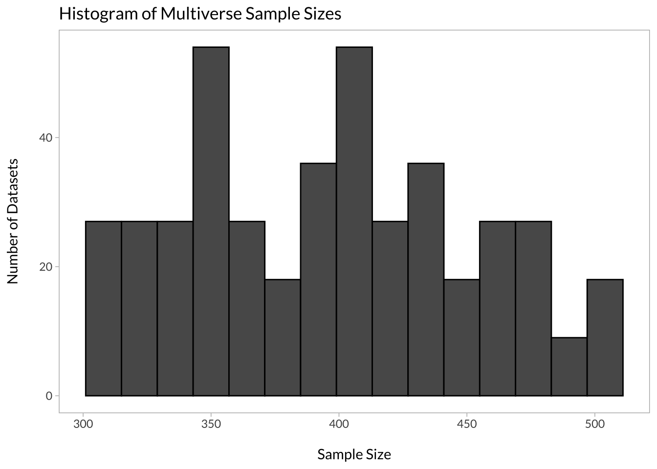
In my case, the minimum sample size was 304 and the maximum was 500. We can also look at which data processing decisions affected sample size the most:
# boxplots showing how sample sizes look across different decisions
mulitverse_sample_size %>%
  select(-ends_with("exp")) %>%
  gather(variable, exclusion, -decision, -n) %>%
  mutate(variable = str_replace(variable, "_(name)$|_(variable_group)$", ".\\1\\2")) %>%
  separate(variable, c("var","group"), sep = "\\.") %>%
  spread(group, exclusion) %>%
  arrange(decision, variable_group) %>%
  ggplot() +
  geom_boxplot(aes(x = name, y = n), notch = T, width = .5)  +
  scale_x_discrete("Exclusion Criteria") +
  scale_y_continuous("Sample Size (max = 500)\n") +
  ggtitle("Sample Sizes in the Multiverse") +
  facet_wrap(~variable_group, scales = "free", ncol = 2)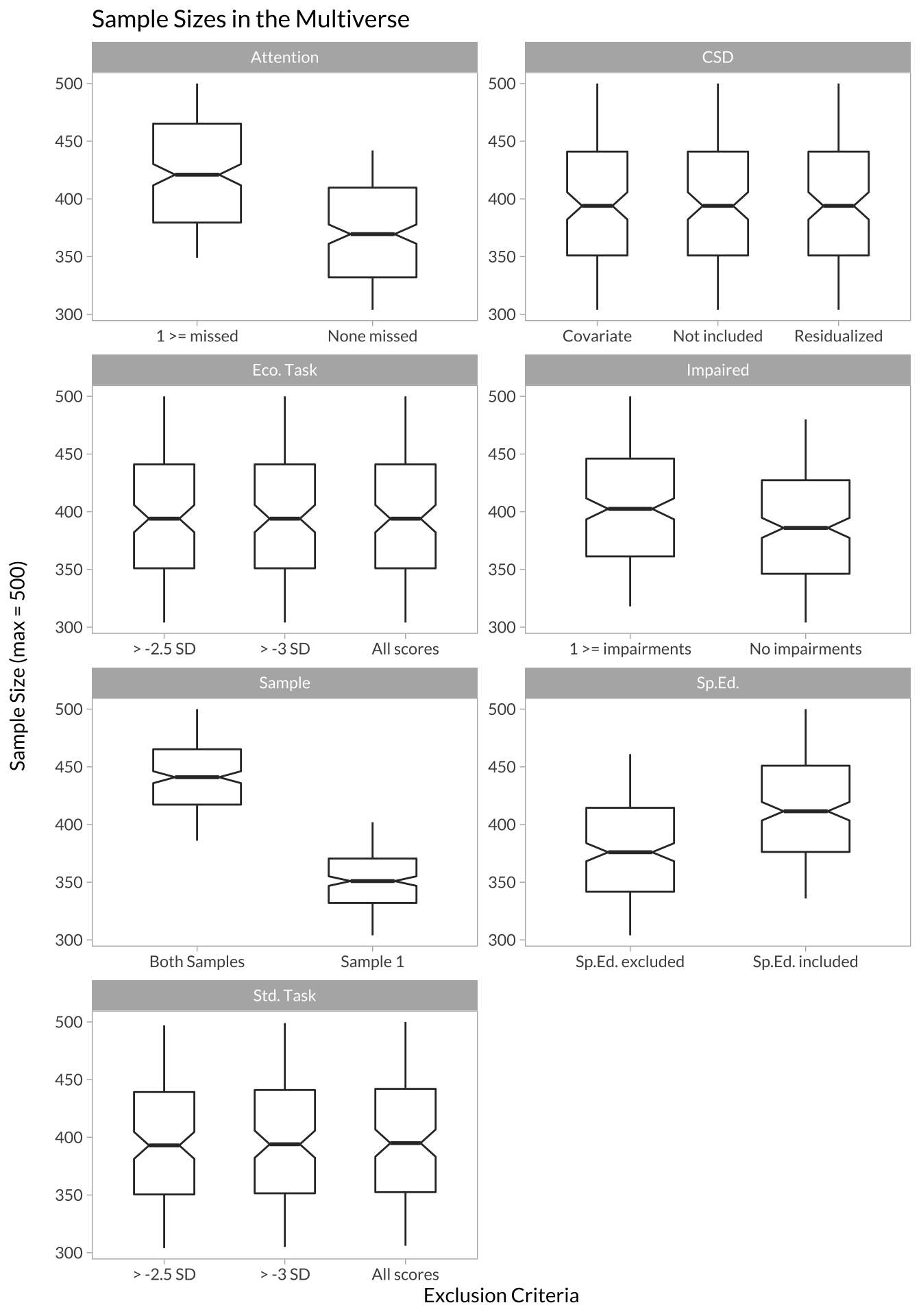
Analyze the Multiverse
I’ve generated our multiverse of datasets, now I need to analyze it. My strategy is to loop over my multiverse_data object. First, I extract the decisions that produced the data to know what we should do with ex_csd (i.e., create residualized scores, include it as a covariate, or do nothing).
Next, I restructure the data into long format so I can run a mixed model with random intercepts to look at the main effect of iv_unp (between-subjects), main effect of task_type (standard or ecological version, within-subjects), and their interaction.
After running the mixed model, I also do a simple slopes test to evaluate (in the context of an interaction) the simple effects of high versus low unpredictability and standard versus ecological versions of the test.
At the end of each iteration, I compile another list with the following components:
- The data
- The decisions that produced the data
- What was done with
ex_csd - The entire mixed model object (e.g.
lmerobject) - The simple slopes test object
- A tidied table of the coefficients from the model
- A table of predicted effects based on +/- 1 SD of
iv_unpandtask_type(standard or ecological) to visualize interactions
# get multiple cores going again
plan(multisession, workers = cores-2)
# Loop through all the datasets in the multiverse and do the same analysis
multiverse_models <-
  future_map(multiverse_data, function(x){
    # Get the expression that produced the data
    decisions <- x$decisions
    csd_decision <- x$decisions %>% filter(variable == "ex_csd") %>% pull(exp)

    # What to do with ex_csd
    nothing <- csd_decision == "0"
    residualize <- csd_decision == "1"
    covariate <-  csd_decision == "2"

    # restructure the data for mixed model
    data <- x$data %>%
      select(-intercept) %>%
      mutate(iv_unp_z = scale(iv_unp) %>% as.numeric()) %>%
      gather(task_type, score, -id, -iv_unp, -iv_unp_z, -starts_with("ex")) %>%
      mutate(task_type = ifelse(task_type=="dv_std", -1, 1)) %>%
      arrange(id, task_type)

    # Should ex_csd be partialed out of the IV?
    if(residualize){
      data_resids <- data %>% distinct(id,ex_csd,iv_unp_z)
      mod_residualized <- lm(iv_unp_z ~ ex_csd, data = data_resids)

      data_resids <-
        broom::augment(mod_residualized, data = data_resids) %>%
        rename(iv_unp_resid = .resid) %>%
        select(id, iv_unp_resid)

      data <- left_join(data, data_resids, by = "id") %>%
        mutate(iv_unp_resid_z = scale(iv_unp_resid) %>% as.numeric())

      mod <- lmer(score ~ task_type*iv_unp_resid_z + (1|id), data = data)
      mod_effects <- ggpredict(mod, terms = c("iv_unp_resid_z [-1,1]", "task_type [-1,1]"))
    }

    # Should ex_csd be used as a covariate?
    if(covariate){
      mod <- lmer(score ~ task_type*iv_unp_z + ex_csd + (1|id), data = data)
      mod_effects <- ggpredict(mod, terms = c("iv_unp_z [-1,1]", "task_type [-1,1]"))
    }

    # Do not do anything with ex_csd
    if(nothing){
      mod <- lmer(score ~ task_type*iv_unp_z + (1|id), data = data)
      mod_effects <- ggpredict(mod, terms = c("iv_unp_z [-1,1]", "task_type [-1,1]"))
    }

    # Simple slopes test for Unpredictability and task type
    if(residualize){
      mod_ss_unp <- sim_slopes(mod, pred = "task_type",  modx = "iv_unp_resid_z", modx.values = c(-1,1))
      mod_ss_task <- sim_slopes(mod, pred = "iv_unp_resid_z", modx = "task_type", modx.values = c(-1,1))
    } else{
      mod_ss_unp <- sim_slopes(mod, pred = "task_type", modx = "iv_unp_z", modx.values = c(-1,1))
      mod_ss_task <- sim_slopes(mod, pred = "iv_unp_z", modx = "task_type", modx.values = c(-1,1))
    }

    # Get the results and turn them into a data.frame
    mod_tidy <-
      mod %>%
      broom.mixed::tidy() %>%
      rename_all(~paste0("mod_",.))

    # Return a list of everything useful
    list(
      data           = data,
      decisions      = decisions,
      residualized   = residualize,
      covariate      = covariate,
      mod_tidy       = mod_tidy,
      mod_sim_slopes = list(unp = mod_ss_unp, task = mod_ss_task),
      mod_effects    = mod_effects
    )
  })
# got back to sequential
plan(sequential)
Multiverse Effect Sizes
With the multiverse of results, I can extract the coefficients (i.e. regression slopes) for plotting and interpretation. Here, I just loop through my multiverse of results to get this information (i.e., fixed main effects and interaction term).
# Get the model estimates out of the giant list
multiverse_estimates <-
  multiverse_models %>%
  map_df(function(x){
    # Grab the decisions flatten them out
    decisions <-
      x$decisions %>%
      gather(key,value,-decision,-variable) %>%
      unite(grid_vars, variable, key) %>%
      spread(grid_vars, value)

    # Add the decisions to the model table
    bind_cols(x$mod_tidy, n = x$n, decisions)
  })
# Only look at our main effects and interaction terms
multiverse_plot_data <-
  multiverse_estimates %>%
  filter(str_detect(mod_term,"^iv_unp_z$|^iv_unp_resid_z$|task")) %>%
  mutate(
    term = str_remove(mod_term,"_resid"),
    term = factor(term,
                  levels = c("iv_unp_z","task_type","task_type:iv_unp_z"),
                  labels = c("Main Effect Unp","Main Effect Task","Interaction")),
    p_value = case_when(mod_p.value <= .05 ~ "p <= .05",
                        mod_p.value >  .05 ~ "p > .05"),
    p_value = factor(p_value, levels = c("p > .05","p <= .05"))
  ) %>%
  group_by(term) %>%
  mutate(multiverse_set = as.numeric(fct_reorder(decision, mod_estimate)))
Displaying the Results
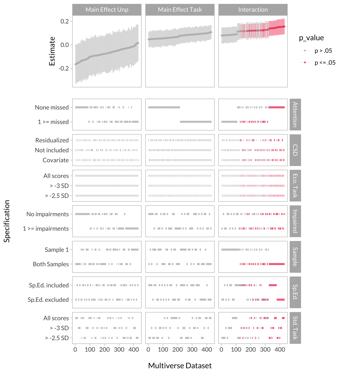
There is a lot of information derived from the multiverse analysis. An efficient way of looking at the results is to visualize the effect size curve and specification grid. The effect size curve involves extracting the effect sizes from each term and arrange them from smallest to largest, and color them by significance. The specification grid (i.e., decisions) is simply a chart indicating which decisions produced the effects in the curve.
Another way to evaluate the results is to create histograms of the p-values for each effect. If the p-values of a particular effect tend to cluster around the set alpha level (usually p < .05), the model is relatively robust to the (arbitrary) data processing decisions. If the distribution looks more uniform, the model is more sensitive to these decisions.
Lastly, because I am primary interested in interactions, I want to plot the form of each interaction obtained. I can do that by plotting predicted estimates based on high and low unpredictability and task-type for every model, coloring lines based on the significance of the interaction term.
Effect Size Curve
multiverse_effect_curve <-
  multiverse_plot_data %>%
  ggplot(aes(x = as.numeric(multiverse_set), y = mod_estimate, color = p_value)) +
  geom_point(size = .5) +
  geom_errorbar(
    aes(x = as.numeric(multiverse_set), ymin = mod_estimate - mod_std.error, ymax = mod_estimate + mod_std.error, color = p_value),
    size = .25,
    width = 0,
    alpha = .25,
    inherit.aes = F,
    show.legend = T
  ) +
  scale_y_continuous("Estimate") +
  scale_color_manual(values = c("gray","#f0506e")) +
  scale_fill_manual(values = c("gray","#f0506e")) +
  facet_wrap(~term) +
  theme(
    axis.text.x = element_blank(),
    axis.title.x = element_blank(),
    axis.ticks.x = element_blank()
  )
multiverse_effect_curve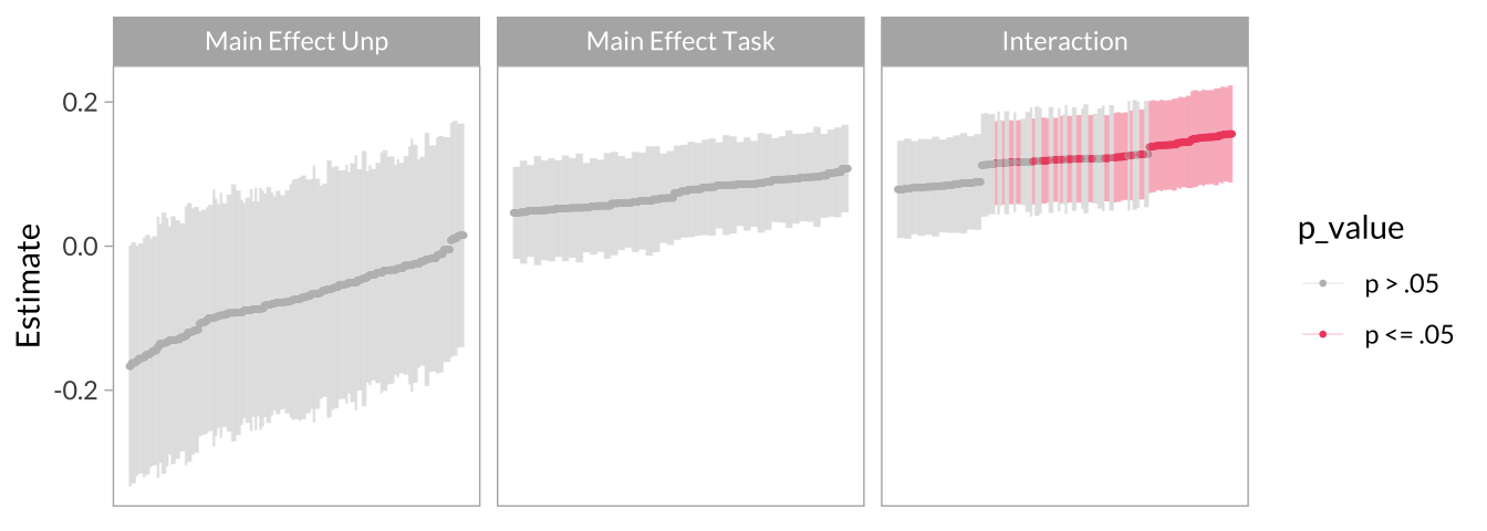
Specification Grid
multiverse_spec_grid <-
  multiverse_plot_data %>%
  select(-matches("exp$")) %>%
  gather(variable, spec, matches("name|group$"), -starts_with("mod"), -decision, -multiverse_set) %>%
  mutate(variable = str_replace(variable, "_(name$)|_(variable_group$)",".\\1\\2")) %>%
  separate(variable, c("variable","group"), sep = "\\.") %>%
  spread(group,spec) %>%
  ggplot(aes(x = multiverse_set, y = name, color = p_value)) +
  geom_point(size = .75, shape = 124, show.legend = F) +
  scale_y_discrete("Specification\n") +
  scale_x_continuous("\nMultiverse Dataset") +
  scale_color_manual(values = c("gray","#f0506e")) +
  facet_grid(variable_group~term, scales = "free_y") +
  theme(strip.background.x = element_blank(), strip.text.x = element_blank(), strip.placement = "outside")
multiverse_spec_grid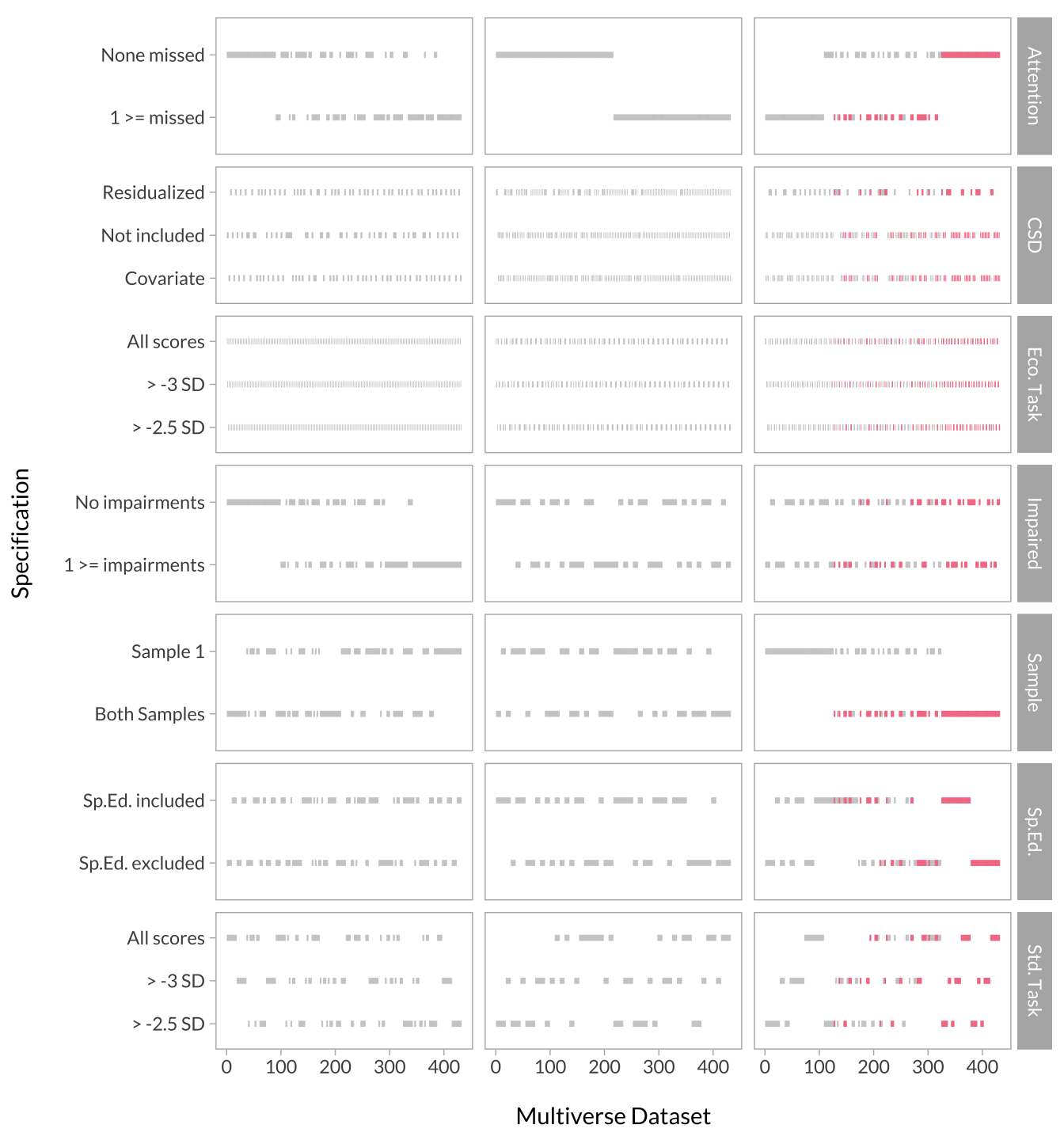
Creating the Full Multiverse Plot
cowplot::plot_grid(
  multiverse_effect_curve,
  multiverse_spec_grid,
  ncol = 1,
  align = 'v',
  axis = "lr",
  rel_heights = c(.25,.75)
)
The Histogram of p-values
multiverse_plot_data %>%
  ggplot(aes(x = mod_p.value)) +
  geom_histogram(color = "black") +
  geom_vline(aes(xintercept = .05), color = "red", linetype = "dotted") +
  scale_x_continuous("\nMultiverse p-value") +
  scale_y_continuous("Count") +
  facet_wrap(~term, scales = "free_y")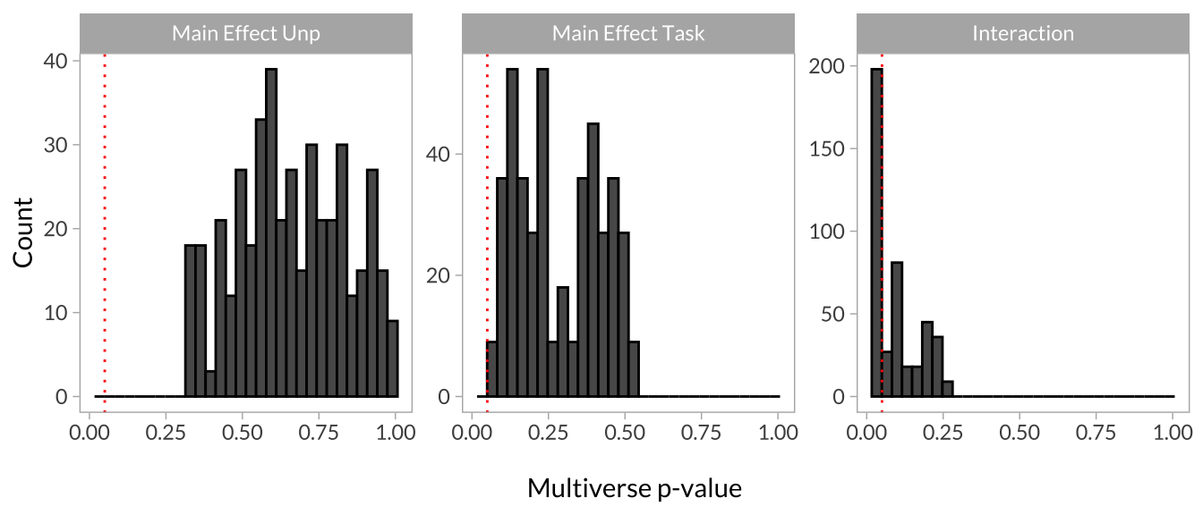
Simple Slopes Effect Curves
These curves are, in principle, the same as the effect size curves above. The difference is that the effect size of interest is a simple slope instead of a regression coefficient from the mixed model. There are four simple effects of interest:
- The effect of task type when unpredictability is low
- The effect of task type when unpredictability is high
- The effect of unpredictability on the standard version
- The effect of unpredictability on the ecological version
The code below grabs this information from our multiverse analysis so I can visualize these effects. Note that I could also make a specification grid for each of these plots but I opted not to for brevity.
# Get the simple slopes tests from our giant list
multiverse_ss <- map_df(multiverse_models, function(x){
  decisions <- x$decisions %>%
    gather(key,value,-decision,-variable) %>%
    unite(grid_vars, variable, key) %>%
    spread(grid_vars, value)

  simple_slopes <-
    bind_rows(
      x$mod_sim_slopes$unp$slopes %>%
        rename_all(~c("value", "slope", "se","lower","upper","t.value","p.value")) %>%
        mutate(group = "unp"),
      x$mod_sim_slopes$task$slopes %>%
        rename_all(~c("value", "slope", "se","lower","upper","t.value","p.value")) %>%
        mutate(group = "task"),
    )

  bind_cols(simple_slopes, decisions)
}) %>%
  mutate(simple_slope = case_when(group=="unp" & value ==  1 ~ "High Unp",
                                  group=="unp" & value == -1 ~ "Low Unp",
                                  group=="task" & value ==  1 ~ "Ecological",
                                  group=="task" & value == -1 ~ "Standard"),
         simple_slope = factor(simple_slope, levels = c("Low Unp","High Unp", "Standard", "Ecological")),
         p_value = case_when(p.value <= .05 ~ "p <= .05",
                             p.value >  .05 ~ "p > .05"),
         p_value = factor(p_value, levels = c("p > .05","p <= .05")))
Unpredictability
This plot shows the effect of task type when unpredictability is low versus high.
multiverse_ss %>%
  filter(group == "unp") %>%
  group_by(group, value) %>%
  mutate(multiverse_set = as.numeric(fct_reorder(decision, slope))) %>%
  ggplot(aes(x = multiverse_set, y = slope, color = p_value)) +
  geom_point() +
  scale_x_continuous("\nMultiverse") +
  scale_y_continuous("Estimate\n") +
  scale_color_manual(values = c("gray","#f0506e")) +
  scale_fill_manual(values = c("gray","#f0506e")) +
  facet_wrap(~simple_slope)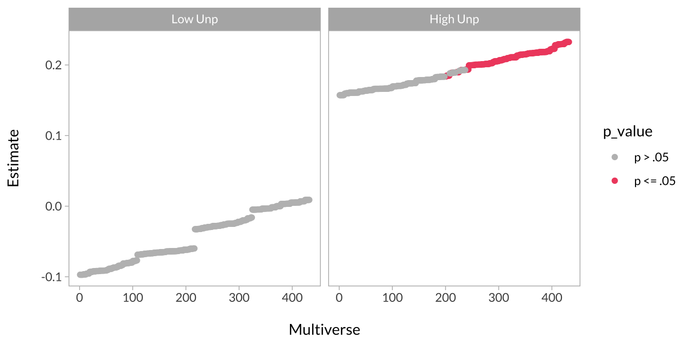
Task Type
This plot shows the effect of unpredictability when task type is the standard versus ecological version.
multiverse_ss %>%
  filter(group == "task") %>%
  group_by(group, value) %>%
  mutate(multiverse_set = as.numeric(fct_reorder(decision, slope))) %>%
  ggplot(aes(x = multiverse_set, y = slope, color = p_value)) +
  geom_point() +
  scale_x_continuous("\nMultiverse") +
  scale_y_continuous("Estimate\n") +
  scale_color_manual(values = c("gray","#f0506e")) +
  scale_fill_manual(values = c("gray","#f0506e")) +
  facet_wrap(~simple_slope)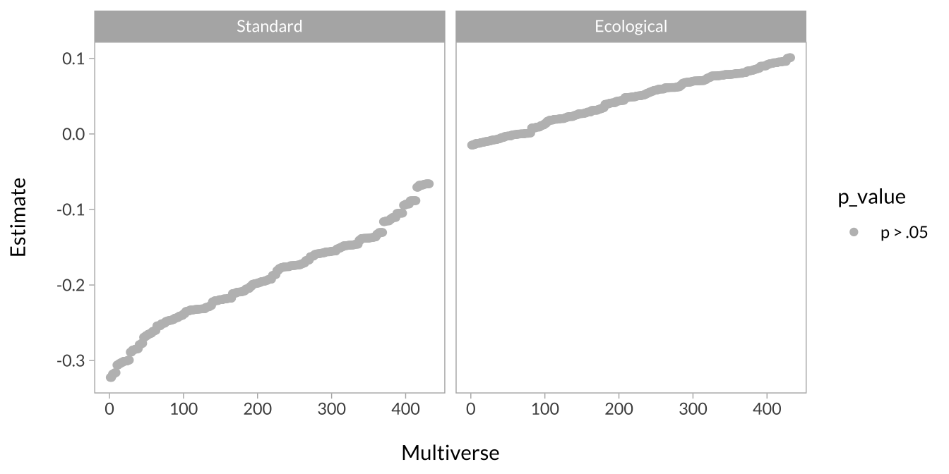
Interaction plots
Here, I simply plot interactions based on high versus low unpredictability and task-type. More specifically, the predicted level of performance when unpredictability is high versus low and on the standard versus ecological version.
Each line represents an interaction from a single dataset in the multiverse. I’ve broken the plots out into panels so the overall pattern is more visible. I’ve also made one plot with unpredictability on the x-axis and separate panels for task type. I made another plot with these flipped.
# Get the predicted points out of our giant list
multiverse_effects <- map_df(multiverse_models, function(x){
  decisions <- x$decisions %>%
    gather(key,value,-decision,-variable) %>%
    unite(grid_vars, variable, key) %>%
    spread(grid_vars, value)

  bind_cols(x$mod_effects, n = x$n, decisions)
}) %>%
  left_join(
    multiverse_plot_data %>% filter(str_detect(mod_term,"\\:")) %>% select(term, p_value, decision),
    by = "decision"
  )
Effect of Unpredictability Across Task Type
# Plot the interactions
multiverse_effects %>%
  mutate(group = factor(group, levels = c(-1,1), labels = c("Standard Version","Ecological Version"))) %>%
  ggplot(aes(x = x, y = predicted, group = decision, color = p_value)) +
  geom_line(alpha = .25,size = .25, show.legend = F) +
  scale_x_continuous("\nEnvironmental Unpredictability") +
  scale_y_continuous("Performance\n") +
  scale_color_manual(values = c("gray","#f0506e")) +
facet_wrap(~group) 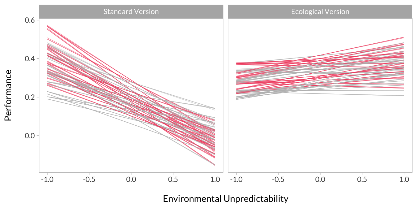
Effect of Task Type Across Unpredictability
# Plot the interactions
multiverse_effects %>%
  mutate(
    group_jitter = jitter(as.numeric(group), amount = .1),
    group        = factor(group, levels = c(-1,1), labels = c("Standard Version","Ecological Version")),
    x            = factor(x, levels = c(-1,1), labels = c("Low Unpredictability","High Unpredictability"))
  ) %>%
  ggplot(aes(x = group_jitter, y = predicted, group = decision, color = p_value)) +
  geom_line(alpha = .25,size = .25, show.legend = F) +
  geom_point(alpha = .25,size = .25, show.legend = F) +
  scale_x_continuous("\nTask Type", breaks = c(1,2), labels = c("Standard","Ecological")) +
  scale_y_continuous("Performance\n") +
  scale_color_manual(values = c("gray","#f0506e")) +
facet_wrap(~x) 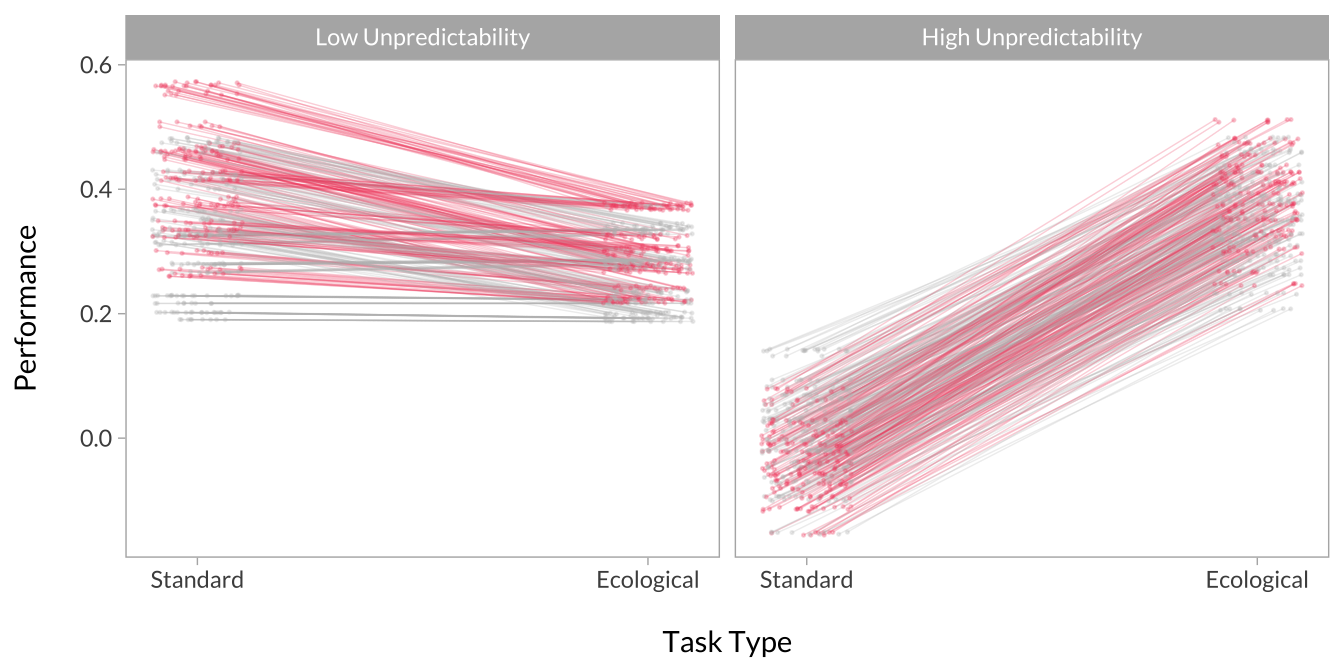
And that’s it! My first foray into multiverse style analysis.